The introduction and application of convolutional neural networks are introduced in detail with Omdan

â–ŒIntroduction

Regarding convolutional neural networks from traffic light recognition to more practical applications, I often hear the question: "Will there be a deep learning "magic" that can judge the quality of food using only images as a single input Bad?" In short, what is needed in business is this:

When entrepreneurs face machine learning, they think this way: Omdan’s "quality" is good.

This is an example of an ill-posed problem: whether the solution exists, whether the solution is unique and stable is not yet certain, because the definition of "done" is very vague (let alone realized). Although this article is not about efficient communication or project management, one thing is necessary: ​​never make a commitment to a project without a clear scope. To solve this ambiguity problem, a good way is to build a prototype model first, and then focus on the architecture for completing subsequent tasks. This is our strategy.

â–ŒProblem definition

In my prototype implementation, I focused on omelette, and built a scalable data pipeline that outputs the perceived "quality" of fried eggs. It can be summarized like this:

Problem type: multi-category classification, 6 discrete quality categories: [good, broken_yolk, overroasted, two_eggs, four_eggs, misplaced_pieces].

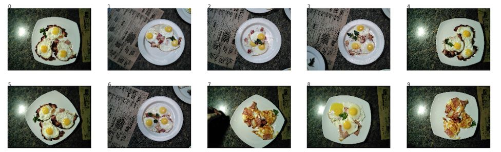
Data set: A variety of omelettes taken by 351 DSLR cameras are manually collected, among which: the training set contains 139 images; the test set during training contains 32 images; the test set contains 180 images.

Tags: Each photo is marked with a subjective quality level.

Metric: Classification cross entropy.

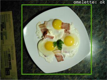
Necessary knowledge: three egg yolks are not broken, some bacon and parsley, no burnt or broken food, can be defined as "good" fried eggs.

Finished definition: The best cross entropy generated on the test set after two weeks of prototype design.

Visualization of results: t-SNE algorithm for low-dimensional data display on the test set.

Input image captured by camera

The main goal of this paper is to use a neural network classifier to obtain the extracted signals, and to fuse them, so that the classifier can make softmax predictions on the class probability of each item on the test set. Here are some of the signals we extracted and found useful:

Key component mask (Mask R-CNN): Signal #1.

Key component counts grouped by each component (basically a matrix of different component counts): Signal #2.

Remove the RGB color and background of the omelette tray and do not add it to the model. This is more obvious: just use the loss function to train a convolutional network classifier on these images, and embed a low-dimensional L2 distance between the selected model image and the current image. But this training only used 139 images, so this hypothesis cannot be verified.

â–ŒGeneral 50K Pipeline Overview (50K Pipeline Overview)

I omitted several important steps, such as data discovery and exploratory analysis, baseline and MASK R-CNN's active labeling pipeline (this is the name I gave to the semi-supervised example annotations, inspired by Polygon-RNN demo video-https ://?v=S1UUR4FlJ84). The 50K pipeline view is as follows:

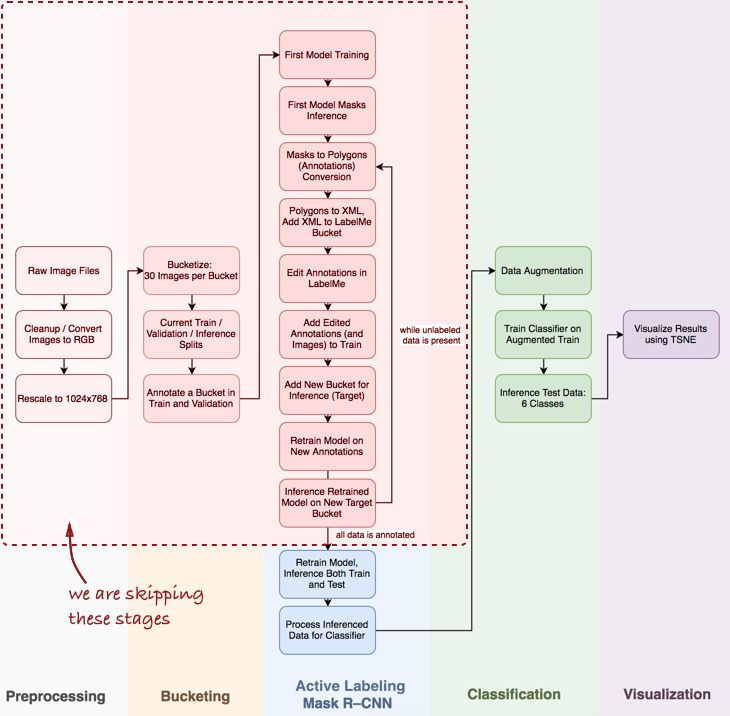
Mask R-CNN and the classification steps of the pipeline

There are three main steps: [1] MASK R-CNN for component mask inference, [2] Keras-based convolutional network classifier, [3] visualization of the result data set of the t-SNE algorithm.

Step 1: Mask R-CNN and mask inference

Mask R-CNN has become more popular recently. From the initial Facebook's paper, to the Data Science Bowl 2018 on Kaggle, MASK R-CNN proved its powerful architecture, such as segmentation (object-aware segmentation). The Keras-based MRCNN code used in this article is well-structured, well-documented, and works fast, but the speed is slower than expected.

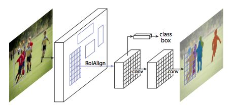
The MRCNN framework shown in the latest paper

MRCNN consists of two parts: the backbone network and the network head, which inherits the Faster R-CNN architecture. Whether it is based on the Feature Pyramid Network (FPN) or ResNet 101, the convolutional backbone network is the feature extractor of the entire image. Above this is the Region Proposal Network (RPN), which samples the region of interest (ROI) for the head. The head of the network performs bounding box identification and mask prediction for each ROI. In this process, the RoIAlign layer finely matches the multi-scale features extracted by RPN with the input content.

In practical applications, especially in prototype design, the pre-trained convolutional neural network is the key. In many practical scenarios, data scientists usually have a limited number of annotated data sets, and some do not even have any annotations. In contrast, a convolutional network requires a large number of labeled data sets to converge (for example, the ImageNet data set contains 1.2 million labeled images). This is where transfer learning is needed: freezing the weights of the convolutional layer, and only retraining the classifier. For small data sets, freezing the convolutional layer weights can avoid overfitting.

The sample obtained after one (epoch) training is shown in the following figure:

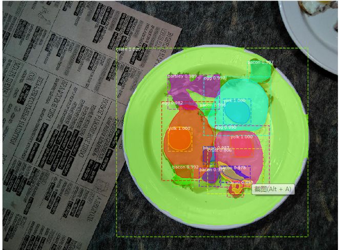
Result of instance segmentation: all key components are detected

The next step is to cut out the dish and extract a two-dimensional binary mask for each component from it:

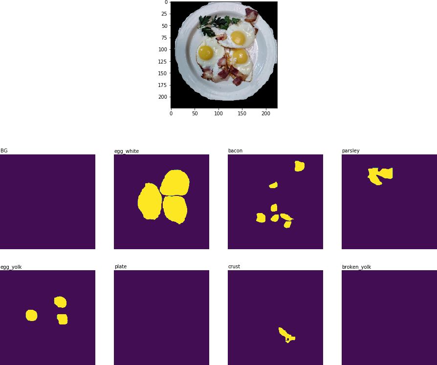
With target plate and key components like binary mask

These binary masks then form an 8-channel image (MRCNN defines 8 mask categories). Signal #1 is shown in the figure below:

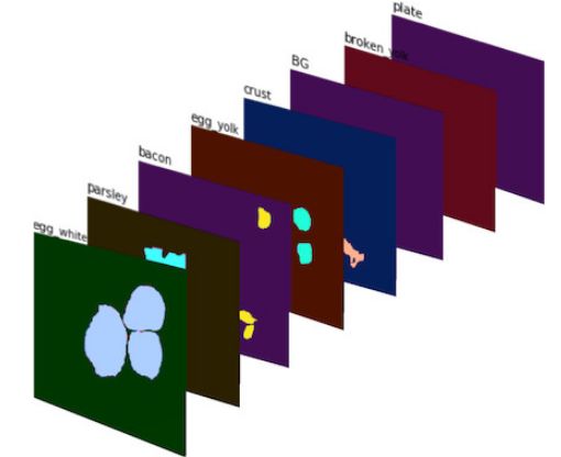
Signal #1: 8-channel image composed of binary mask. The different colors are just for better visual observation.

For Signal #2, MRCNN infers the amount of each component and packs it into a feature vector.

Step 2: Keras-based convolutional neural network classifier

We have built a CNN classifier from scratch using Keras. The goal is to integrate several signals (Signal#1 and Signal#2, more data will be added in the future) and let the network make predictions about the quality of food categories. The real architecture is as follows:

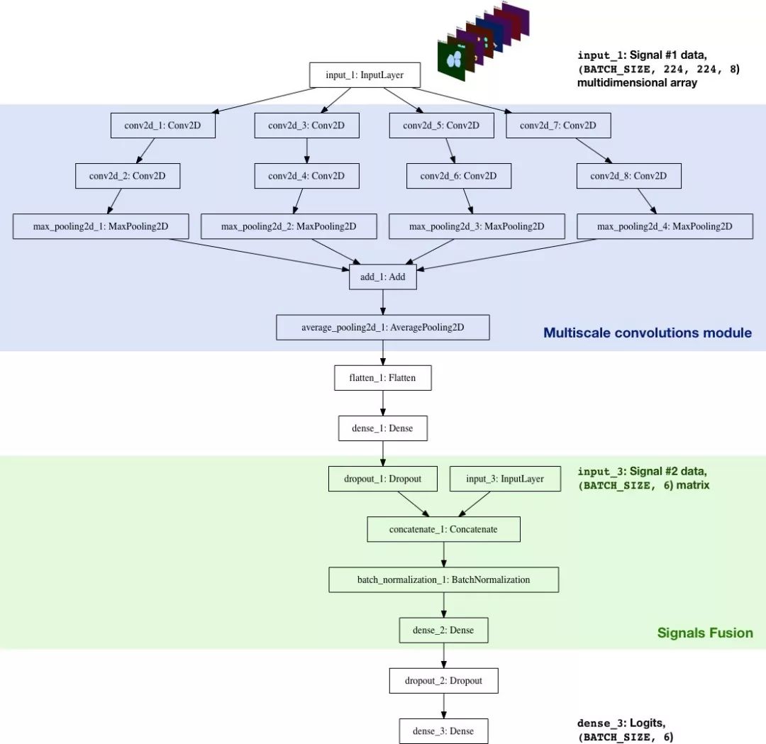
The characteristics of the classifier architecture are as follows:

Multi-scale convolution module: Initially, the kernel size of the convolution layer was 5*5, and the result was not satisfactory, but there are several convolution layers with different kernels (3*3, 5*5, 7*7, 11*11) AveragePooling2D works better. In addition, a 1*1 convolutional layer is added before each layer to reduce the dimensionality, which is similar to the Inception module.

Larger kernel: A larger kernel is easier to extract a larger range of features from the input image (itself can be regarded as an activation layer with 8 filters: the binary mask of each part is basically a filter) .

Signal integration: The model only uses a nonlinear layer for two feature sets: the processed binary mask (Signal#1) and the number of components (Signal#2). Signal#2 increased cross entropy (increased cross entropy from 0.8 to [0.7, 0.72]))

Logits: In TensorFlow, this is the layer where tf.nn.softmax_cross_entropy_with_logits calculates the batch loss.

Step 3: Use t-SNE to visualize the results

Use t-SNE algorithm to visualize the results, which is a popular data visualization technology. t-SNE minimizes the KL divergence between the joint probability of the low-dimensional embedded data points and the original high-dimensional data (using a non-convex loss function).

In order to visualize the classification results of the test set, I exported the test set image, extracted the logits layer of the classifier, and applied the t-SNE algorithm to the result data set. The effect is quite good, as shown in the following figure:

Visualization of the t-SNE algorithm on the prediction results of the classifier test set

Although the result is not particularly perfect, this method is indeed effective. The areas that need to be improved are as follows:

More data. Convolutional neural networks require a lot of data, and there are only 139 samples used for training. The data enhancement technique used in this article is particularly good (using D4 or dihedral, symmetry to generate more than 2,000 enhanced images). However, if you want a good performance, more real data is especially important.

Appropriate loss function. For simplicity, this article uses the classification cross-entropy loss function. You can also use a more appropriate loss function-triplet loss, which can make better use of intra-class differences.

A more comprehensive classifier architecture. The current classifier is basically a prototype model designed to interpret the input binary mask and integrate multiple feature sets into a single inference pipeline.

Better labels. I'm really bad at manual image labeling (quality in 6 categories): the classifier's performance on more than a dozen test set images exceeded my expectations.

â–ŒReflection

In practical applications, companies have no data, notes, and no clear tasks to complete, but this phenomenon is very common and it is undeniable. This is a good thing for you: all you have to do is to have tools and enough GPU hardware, business and technical knowledge, pre-trained models, and other things of value to the enterprise.

Start with small things: a prototype model that can be built with LEGO code blocks can further improve the efficiency of communication-to provide enterprises with this solution is the responsibility of a data scientist.

AOC Cable

Aoc Cable,Multicore Optical Fiber Connector,Single Mode Optical Fiber Connector,Fiber Optic Network Cable Connector

Dongguan Aiqun Industrial Co.,Ltd , https://www.gdoikwan.com