Mathematical model of the system—differential equations and transmission operators

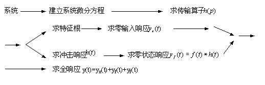
Chapter 2 Time Domain Analysis of Continuous System

It does not involve any mathematical transformation, but directly analyzes the system in the time variable domain, which is called the time domain analysis of the system. There are two methods: classical time domain method and time domain convolution method.

The classical method in the time domain is a method to directly solve the differential equations of the system. The advantage of this method is intuitive, the physical concept is clear, the disadvantage is that the solution process is redundant and the application is also limited. Therefore, before the 1950s, people generally like to use transform domain analysis methods (such as the Laplace transform method), and less time classic methods. Since the 1950s, due to the universal application of the δ (t) function and computers, the time-domain convolution method has been rapidly developed, and has continued to mature and improve, which has become one of the important methods of system analysis. The time domain analysis method is the basis of various transform domain analysis methods.

In this chapter, first establish the mathematical model of the system-the differential equation, then use the classical method to find the zero input response of the system, use the time-domain convolution method to find the zero state response of the system, and then add the zero input response to the zero state response Get the full response of the system. The ideas and procedures are:

Next, we will introduce: the system is equivalent to a differential equation; the system is equivalent to a transmission operator H (p); the system is equivalent to a signal-impulse response h (t). To analyze the system is to study the relationship between the excitation signal f (t) and the impulse response signal h (t). This relationship is the convolution integral.

2-1 Mathematical model of the system-differential equations and transmission operators

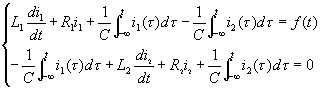
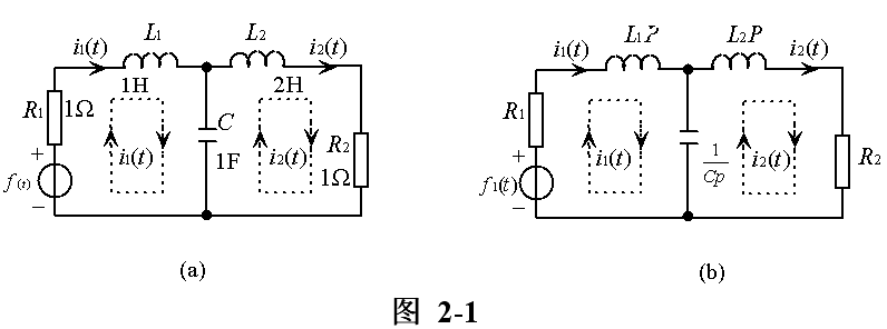
To study the system, we must first establish the mathematical model of the system-differential equations. The basis for establishing the differential equations of a circuit system is the two constraints of the circuit: topological constraints (KCL, KVL) and component constraints (the time-domain volt-ampere relationship of the components). In order to make it easy for readers to understand and accept, we take a special to general method to study.

Figure 2-1 (a) shows a dual-mesh circuit with three independent dynamic components, where To motivate, , In response. For two mesh loops, the KVL equation can be listed as

The above two formulas contain two variables , Simultaneous differential integral equation.

In order to obtain a differential equation containing only one variable,

Differential operator , which is

, , ...,

Differential operator After that, the above differential equation can be written

which is

(2-1)

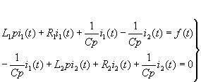
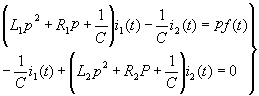
The circuit model in the form of an operator can be drawn according to equation (2-1), as shown in Figure 2-1 (b). Compare Figure 2-1 (a) with (b),

It is easy to draw Figure 2-1 (b) according to Figure 2-1 (a), that is, rewrite L to Lp and C to ,

Everything else remains unchanged. After the operator circuit model is drawn, the equation (2-1) can be easily written according to the operator circuit model column of Fig. 2-1 (b).

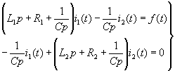
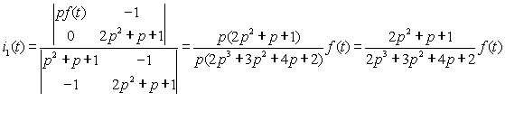
Simultaneously multiply the two ends of the equal sign of equation (2-1) by p at the same time to obtain simultaneous differential equations, ie

Substituting the known data into the above formula, we get

(2-2)

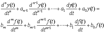
Using the determinant method, the response i1 (t) can be obtained from equation (2-2) as

Note that in the calculation process of the above formula, the common factor p in the numerator and denominator is eliminated. This is because the circuit under study is third-order,

Therefore, the differential equation of the circuit should also be third-order. However, it should be noted that the common factors in the numerator and denominator are not eliminated under any circumstances.

Some situations can be eliminated, while others cannot, depending on the specific situation. Therefore

which is

which is

The above formula is the third-order linear non-homogeneous ordinary differential equation with constant coefficient i1 (t).

The left end of the equation is the linear combination of the response i1 (t) and its various derivatives,

The right end of the equal sign is the linear combination of the excitation f (t) and its derivatives.

Using the same method, i2 (t) can be obtained as

which is

which is

which is

The above equation is the differential equation describing the relationship between the response i2 (t) and the excitation f (t).

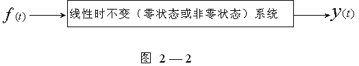
To generalize, for an n-order system, if y (t) is the response variable and f (t) is the excitation, as shown in Figure 2-2, the general form of the system differential equation is

(2-3)

Differential operator Means

Or written as

Can also be written as

In the formula

The characteristic polynomial called system or differential equation (2-3);

(2-4)

H (p) is called the transfer operator or transfer operator of response y (t) to excitation f (t), which is the ratio of two real coefficient polynomials of p,

The denominator is the characteristic polynomial D (p) of the differential equation. H (p) describes the characteristics of the system itself and has nothing to do with the excitation and response of the system.

Here is a point: the letter p is essentially a differential operator, but from the perspective of mathematical form, it can be artificially regarded as

A variable (usually a complex number). In this way, the transmission operator H (p) is the ratio of two real coefficient rational polynomials of p.

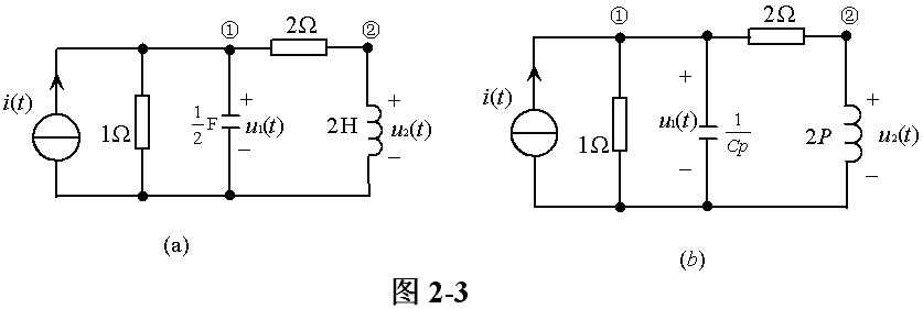
Example 2-1 The circuit shown in Figure 2-3 (a). Find the response u1 (t), u2 (t) to the excitation The transmission operator of u and u1 (t), u2 (t) are the differential equations of i (t) respectively.

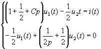
The circuit to solve its operator form is shown in Figure 2-3 (b). For the nodes â‘ , â‘¡ the KCL equation in the form of column operators is

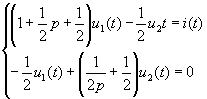
Substitute the data

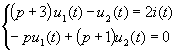
Simultaneously multiply each item of the above formula by p and arrange

Use the determinant method to obtain

Therefore, the transmission operators of u1 (t) to i (t) and u2 (t) to i (t) are:

In turn, u1 (t) and u2 (t) respectively make the differential equations for i (t) as

which is

It can be seen that for different responses u1 (t), u2 (t), the characteristic polynomial Are all the same,

This is the invariance and identity of the system characteristic polynomial.